About FFHedge
What is this?
As the 2026 fantasy football season approached, I (Jon) began considering how I could use Claude Code to build the fantasy football dashboard that I’ve imagined creating for years but never had the bandwidth to bring to life. My main goal was to show how to merge and update information from two sources (“experts” and “data”) into a “blended” Bayesian model to generate weekly predictions as decision-relevant probabilities with uncertainty, while tracking the accuracy of those predictions.
I deliberately kept the two sources as two separate models, combined in the open, rather than folding the expert rank into a single model as one predictor among many; the goal was to see the two signals and where they disagree, not to dissolve them into a list of coefficients. The structure mirrors the informal back-and-forth I run in my head each week, made explicit.
Watch the 3-minute tour
But why?
I have been playing fantasy football for a long time — in my earliest leagues, we drafted teams via email and checked the newspaper for weekly player stats — and I’ve racked up my share of trophies over the years. As I contemplate which players to start or sit on Sunday mornings during the fantasy football season, I find myself running the same calculations in my head. I start with where the expert consensus has each player ranked. A ranking that aggregates dozens of analysts contains valuable wisdom-of-the-crowd signals, and I have learned, repeatedly and sometimes painfully, not to bet against it lightly.
Yet such rankings are not foolproof, even when experts are carefully selected and rankings are calibrated for accuracy (e.g., see FantasyPros “Expert Consensus Rankings” or ECR). For instance, herd mentality, the tendency of some experts to adjust their rankings to be in line with others, might distort useful signals in expert consensus rankings. Relatedly, asymmetric loss functions in predictive accuracy checks might over-penalize experts taking certain types of bold risks, which could bias expert predictions in ways that are misaligned with how I like to make draft or start/sit decisions.
So I may adjust my expectations using player usage or game environment data, nudging a player up because his snap share has been climbing or down because the matchup looks brutal, and somewhere in that informal weighing of consensus against the numbers I arrive at a start-or-sit decision I can live with. This dashboard is an attempt to do that weighing formally, and in public.
It owes a debt to Nate Silver’s The Signal and the Noise, three of whose lessons shaped the whole project. The first is that aggregated forecasts tend to beat individual ones, which is exactly what an expert consensus rank is, and why I treat it with respect rather than suspicion; unless you can foresee the future, your best baseline bet is usually to go with the experts (and flip a coin when it is a close call). The second is that good forecasting means thinking in probabilities and being honest about uncertainty, rather than issuing a single confident number. The third is the Bayesian habit of starting from a sensible prior and updating it as the evidence arrives. The model behind this dashboard takes the expert consensus as that prior and updates it with what the usage and game-environment data are saying, and the rest of the site is about showing you that process instead of hiding it behind a simple list of confident projections.
3 lessons from Silver’s The Signal and the Noise
Before getting into the modeling details, I want to illustrate these three lessons with real examples using WR data from this site. Let’s go with the following common scenario: We are considering two players ranked in the WR3 tier (ECR ≈ 25 to 36) as potential starters in a flex spot. As a fellow NC State alum, Jakobi Meyers will be the recurring star in these examples.
1. Just flip a coin
Many of the start/sit decisions we agonize over weekly in fantasy football could be resolved rationally by simply flipping a coin. For example, in week 12 of 2025, you might have been choosing between Khalil Shakir (ECR = 26) and Jakobi Meyers (ECR = 33):
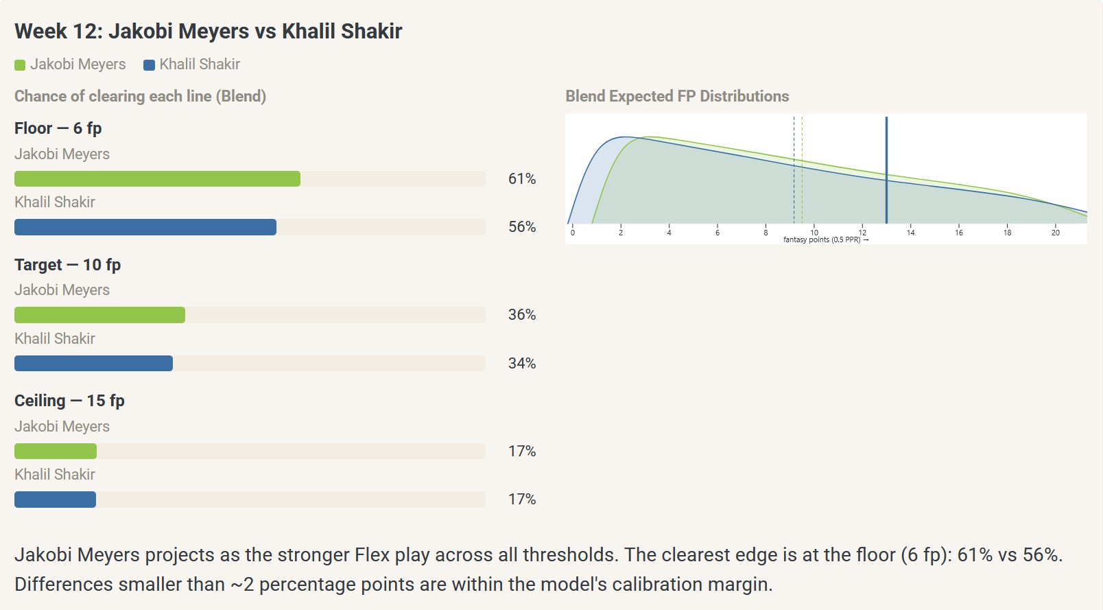
My “Blend” model (more on that later) projected Meyers at a slightly higher probability to clear a minimally useful “floor” scoring threshold of 6fp for a flex starter despite being ranked several spots below Shakir on ECR, but both were approximately coin-flip bets to clear this bar (61% vs. 57%). Meyers and Shakir were projected with a similar probability of clearing the flex target score of 10fp (37% vs. 35%, or about 1-in-3 chance; these are reasonably equivalent considering my model’s 2-percentage-point average error on hold-out probability predictions. Both were predicted as equally unlikely to clear the flex ceiling at about 1-in-5 chance (18% vs. 19%).
Interestingly, both actually scored 13.0 points (cleared flex target) in week 12. This is an exception to the rule: Even when expert consensus places players in the same tier, the variance in what actually happens typically swamps the differences a model can resolve in advance, which is why no projection — Expert, Data, or Blend — is going to get you “the right pick” with confidence on most close calls. Hence, in these cases, where predictions are this close, just go with your gut or flip a coin (and then blame the coin rather than yourself when things go wrong).
2. Use probabilities and uncertainty instead of a single number
Staying with the same week (2025, week 12), what if your decision instead was between Ricky Pearsall (ECR=30) and Jakobi Meyers (ECR=33) at your flex spot? The ECR rankings are closer here, and they slightly favor Pearsall. Let’s check the model predictions:
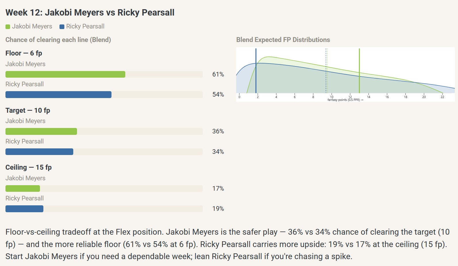
The predicted probabilities of clearing flex scoring thresholds are also relatively similar, so a coin flip is probably warranted here too. However, in this situation, I probably would have felt like I knew what I was getting with Meyers, whereas Pearsall’s lack of data at that point (active weeks 1-4, 11; 1fp in week 11) due to an injury-ridden season would have made me view him as a more volatile play. So, rather than simply relying the single ECR ranking, I would have checked their scoring and usage history, game environment, and my matchup, then approached the decision as one between a relatively stable floor play in Meyers and a slightly higher ceiling play that came at the cost of higher variance (or a noisier signal) in Pearsall. In short, I would have envisioned a somewhat different range of plausible outcomes — or different probability distributions — for both players. Likewise, the Blend model shows a somewhat wider blue predicted fp scoring distribution for Pearsall, with more mass at 0fp and a slightly longer tail at 20+fp, which visually represents him as a lower floor and higher ceiling play.
3. Start from a sensible prior and update with new evidence.
The first two examples were cases where the options were quite similar and the sources of information (expert consensus vs. player usage/game environment data) were relatively well-aligned. However, that is not always the case; sometimes expert consensus and usage/game data predictions diverge. What should we do in such situations? That’s what this site is all about. Let’s illustrate with an example.
In 2025, many experts tagged Travis Hunter as an elite breakout candidate. Of course, everyone wants to draft the next rookie star, and no one wants to pass on, sit, trade, or drop a rookie before their breakout. (Trust me, I know — I drafted and then traded Justin Jefferson before he broke out in his electric rookie season.) Knowing this, some experts might err on the side of bullish predictions for promising rookies even after contradictory data start rolling in.
Yet, compared to later in a season, early season decisions are made under conditions of much greater uncertainty with lots of unknowns, and few decisions are more uncertain than early season rookie projections. Likewise, I tend to be wary of overvaluing rookie potential (at least in redraft leagues), particularly at WR where it is hard to predict breakouts, especially early in their first season. So, in the absence of meaningful usage data from the previous season for rookies, I tend to assume that a starting-caliber rookie WR is more likely to generate league-average production than they are to break out, then I update that assumption as new data emerges.
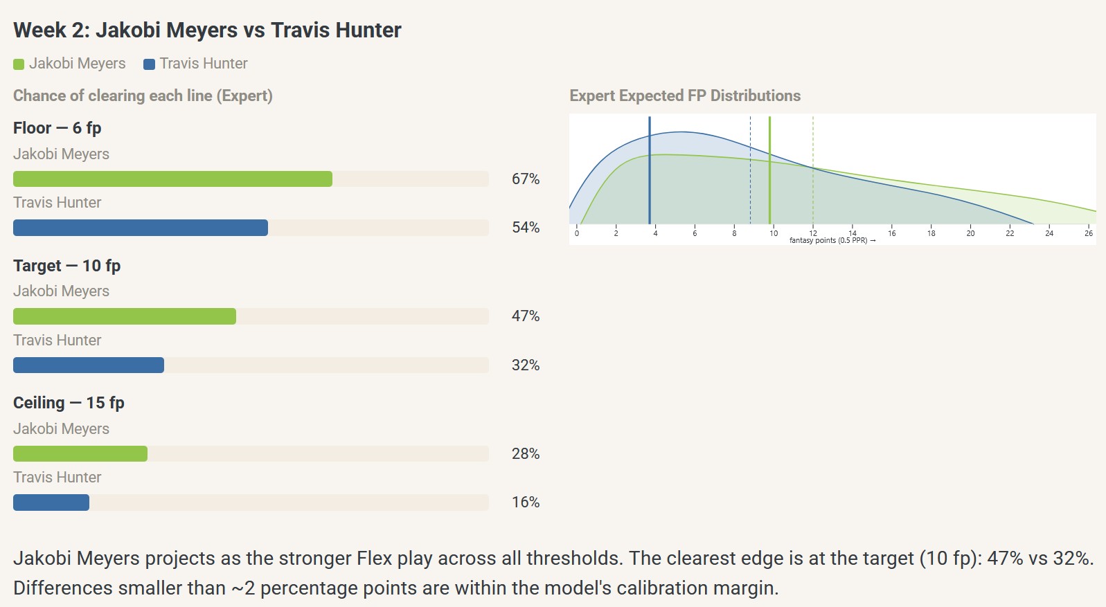
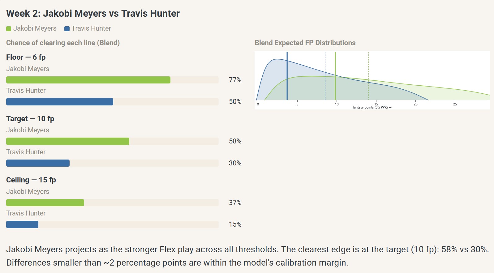
So, in week 2 of 2025, perhaps you were choosing between the stable veteran Jakobi Meyers (ECR = 27) and the electric rookie Travis Hunter (ECR = 31) as a flex starter. At that point, experts had Meyers ranked at a slightly higher ECR, which translated to a 15-percentage-point difference in my model-based probability of exceeding the flex target score (47% vs. 32%):
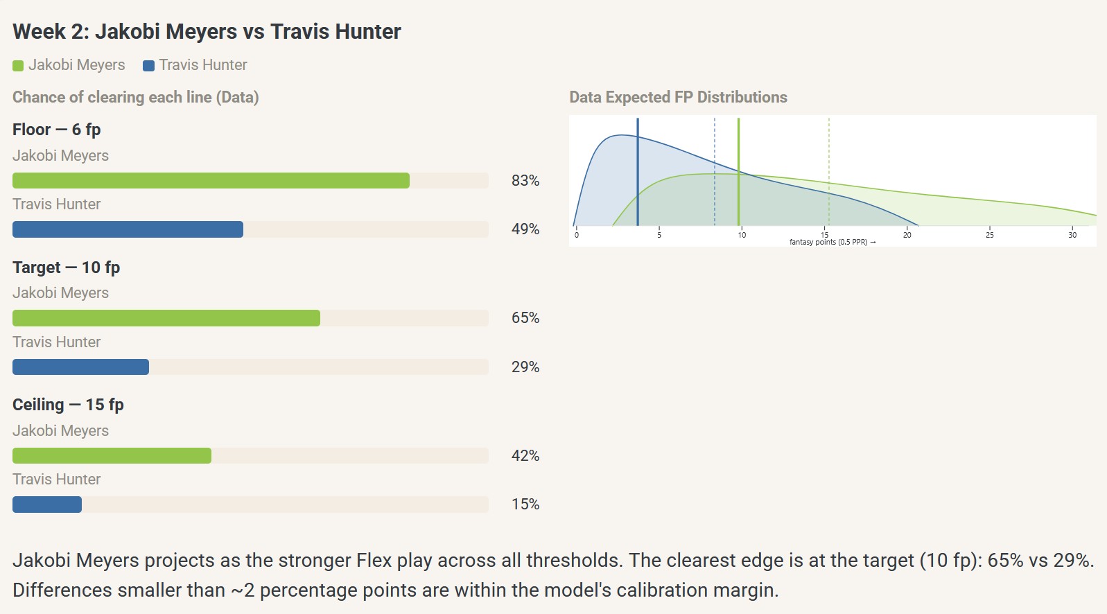
But the player usage/game environment data predictions showed a much larger gap in favor of Meyers, equivalent to a predicted 36-percentage-point difference in the probability of exceeding the flex target score (65% vs. 29%), or a gap more than twice as large as that predicted from the expert-anchored model:
Of course, week 2’s data signal was driven largely by player usage trends observed in week 1. Prior to week 1, experts had Hunter (ECR = 33) ranked ahead of Meyers (ECR = 38). Then, in week 1, Meyers had 8 receptions for 97 yards on 10 targets and 97 air yards (ranked 33rd in air yards); Hunter had 6 receptions for 33 yards on 8 targets and 59 air yards (51st in air yards). That was enough to flip the expert consensus in favor of Meyers (week 2: ECR = 27 for Meyers vs. ECR = 31 for Hunter), but that movement was not enough to match the data model’s much larger predictive gap.
Put differently, expert consensus showed a difference of only four ECR spots, which signals two nearly exchangeable players — flip a coin. Meanwhile, the usage/environment data showed Meyers as a near-lock to clear a usable floor, with a 2-in-3 chance of hitting the flex target and nearly a coin-flip’s chance of a spike week; Hunter, by contrast, had barely a coin-flip chance at clearing as a floor play, a 1-in-3 chance of hitting the flex target, and about a 1-in-7 chance of a spike week.
So, in 2025 week 2, how confident should we have been in Meyers’ superiority as a flex starter over Hunter? Which one should we trust - the experts’ all-things-considered ranking, or the player usage and game environment data? Why choose, when I can hedge my predictions by combining both expert and data models into a “blended” model that merges potentially useful signals from both:
Savvy readers might be thinking: “But, you’re double-counting the data!” After all, the experts already consider player usage metrics and game environment data when they created their rankings, and some apply more sophisticated algorithms than the linear baseline used here, and probably better predictors on their own terms.
Yes, this is true and worth taking seriously. Expert consensus already absorbs much of the usage and game-environment information my data model uses, so the data model on its own mostly retraces ground the experts have covered. What the two-model design offers is a different way of transparently processing mostly the same information: an opaque expert aggregate of many private weightings on one side, and on the other a deliberately minimal, transparent reference point with explicit coefficients on a handful of potential signals. And where the two readings disagree turns out not to be random noise. For example, I found experts systematically under-project fill-in wide receivers by about 1.5 fp, while the data side under-projects returning star receivers by about the same amount. Showing both readings side by side, where they part ways, and how we might combine them to hedge our decisions, is what this site is built to do.
Now that you’ve got a sense of what’s happening here, I’ll briefly walk you through the basic mechanics.
How the Expert, Data, and Blend views are built
As illustrated in the example above, three projections appear throughout this dashboard. Blend is the deployed model. Expert and Data are not separate models set up beside it; they are the two halves of the deployed model itself, which is what makes the comparison between them faithful rather than illustrative.
The deployed model is a stack. Within two distributional families, a zero-inflated negative binomial and a gamma, used because no single family captured both the spike at zero scores and the long right tail, it combines a consensus-anchored model and a usage-driven model, and it then combines the two families. Grouping the pieces of that stack by which model they came from splits the deployed predictive exactly into an expert-driven part and a data-driven part. Expert is the consensus-anchored part, whose dominant input is the published expert consensus recalibrated against past outcomes; Data is the usage-driven part, built from snap share, target share, and game environment. The deployed Blend is an equal, 50/50 average of these two parts, a deliberate hedge rather than a tuned lean, and a slider on the projection pages lets you shift it toward either side.
Two cautions are worth stating plainly. First, the equal split is a choice, not a measurement: when I looked closely, the stacking weights that would have set the lean turned out to be too poorly identified to trust, so the deployed default hedges them evenly and the slider hands the lean to you (the methodology page tells that story). And because experts already draw on usage and matchup information themselves, the Expert view is best understood as human consensus expressed as a predictive distribution rather than as a data-free forecast. Second, every quantity shown here is computed directly from the model’s posterior draws, so the means, the percentiles that shape each curve, and the probability of clearing each roster threshold are all exact, with no post-hoc averaging.
The model, briefly
Under the hood are two deliberately different Bayesian models. One is anchored on the expert consensus, taking the FantasyPros aggregated ECR rank (converted to expected points through a frozen calibration) as its main input and adjusting for injury status and a player-specific history. The other ignores the consensus entirely and works from usage and game environment, things like snap share, target share, and the Vegas-implied game script. Each is fit in two distributional families, a zero-inflated negative binomial and a gamma, because no single family captured both the weeks a player is barely involved and the long upside tail of a smash game. The pieces are combined by stacking, a method for weighting predictive distributions by how well they actually forecast, first within each family and then across them. Everything was locked before the 2025 season was ever examined, and 2025 served as a single held-out test with the predictions registered in advance. The full details, including the pre-registration and the family selection, are on the methodology page.
What I found
A few core results, each shown in full on the page named:
- The experts generally win the ranking, and that is expected. Across 2025, ranking players by raw expert consensus was at least as accurate as the deployed blend on weekly top-12 and top-24 hit rate for receivers and backs; for tight ends the blend roughly matched, even slightly edged, the consensus, and for quarterbacks it drew even — the positions where it held its own on ranking. The model was never built to out-rank a wisdom-of-the-crowd signal, but it should compete favorably while providing useful predicted probabilities and plausible outcome (uncertainty) distributions; see Track Record.
- The probabilities are well-calibrated. The model’s stated chances of clearing a line track observed frequencies closely — within roughly two to three percentage points for receivers, backs, and quarterbacks. Tight ends are the softest of the four, around two to six points and widest at the floor, where tight-end scoring is spikiest; see Track Record.
- The hedge pays off where it should. The cost of full uncertainty distributions and calibrated probabilities is that the blend rarely wins a single week outright; however, it posts similar or even lower CRPS over the season for every position — and for tight ends the lowest of the three sources outright — the payoff of not having to guess in advance whether the experts or the data will be closer; see Track Record.
- Where the experts and the data disagree, the disagreement is mostly noise. I went looking for systematic situational blind spots and, on careful scrutiny, did not find ones that held up, which is itself a reason to hedge rather than chase either signal’s outliers; see Edge Finder.
- A bigger disagreement is not a better signal. When either expert or data model is the dramatic outlier, it is usually the one over-reaching; see Edge Finder.
Those last results fit together better than it might first appear. The experts win the ranking and yet the equal-weighted blend posts similar or lower CRPS, which can look like a contradiction and is not. Ranking and calibrated forecasting are different jobs: a model can lose the race to order players and still produce better-shaped probability distributions, and that is exactly what the hedge does, buying calibration and a lower CRPS rather than a sharper top-12 list. Since much of what the experts see already shows up in a productive player’s usage, holding the two halves evenly costs little on the ranking while gaining on the distribution. The experts are the slightly better ranker; the blend is tuned to be an accurate forecaster of uncertainty. Both are true at once, and holding them both in view is the whole point of the dashboard.
I started with wide receivers, then extended the same two-model, two-family, stacked design to running backs, tight ends, and quarterbacks, each trained on 2022 through 2024 and tested on the sequestered 2025 season exactly as the receiver model was. Each added its own character: the running-back stacking leaned even harder toward usage than the receiver one, which is part of what convinced me the lean was noise rather than signal, and the tight-end stacking leaned almost entirely on the discrete zero-inflated family, the right shape for a low-scoring, boom-or-bust position, and the quarterback stacking leaned the other way, mostly onto a continuous family that suits a high-scoring position with a small genuine negative tail. Deployed as the same equal hedge, both hold up well on calibration and post an equivalent or lower CRPS than either half alone, while — like the receiver model — ceding the pure ranking task to the expert consensus, though tight end comes closest to matching it. Tight end and quarterback each ship a single startable tier rather than the WR1/WR2 split — tight end because it is too top-heavy for a coherent middle, quarterback because you start only one and it never flexes. The position control on each page switches between quarterbacks, wide receivers, running backs, tight ends, and a combined flex pool, and the full account for each position is on the methodology page.
Limitations and next steps
This is a proof of concept with real limits, and naming them is also part of the point. It covers wide receivers, running backs, tight ends, and quarterbacks, on a half-PPR scoring scale. It was tested on a single held-out season, so the results, especially the situational findings drawn from small numbers of fill-in or returning-star weeks, should be read as suggestive rather than settled. The Expert, Data, and Blend views are model-based summaries rather than the raw numbers experts publish, as the section above explains. And the consensus signal is a rank converted to points through a fixed mapping, not a set of published point projections, since I could not find a free archive of stably constructed historical weekly projections. None of this undercuts the approach; it bounds what the numbers can claim.
Given enough data, a natural next step might be to let the expert-versus-data weighting vary by player situation (e.g., stable veteran; returning star; fill-in) rather than holding it fixed, since the held-out results suggest the right balance is not the same for a returning star as for a fill-in. More immediate and obvious next steps are to add alternative scoring options (e.g., standard and full PPR), additional out-of-sample validation by backtesting older seasons rather than resting on a single held-out year, and to carry the predictions forward to a live upcoming (e.g., 2026) season.
Data and acknowledgments
All player statistics, schedules, snap counts, injury reports, and Vegas lines come from the nflverse project via the nflreadr package, released under a CC-BY-SA-4.0 license; the data and any derivatives shared here carry the same license. The expert consensus rank is the FantasyPros aggregated ranking, retrieved through the nflverse archive. This is a non-commercial, educational project, and the FantasyPros rankings are used here only as an analytical signal, not redistributed as a standalone product.
The dashboard and the model behind it were built with the assistance of Claude Code.
Colophon
Built by Jon Brauer as a side project of reluctant criminologists. Questions and corrections are welcome at reluctantcrim@gmail.com.